The idea
A maze is a spanning tree of a grid. Every cell is a vertex, every
pair of orthogonally adjacent cells is a candidate edge, and carving a
passage means keeping that edge. generate_maze() offers
five classic ways to build such a tree, chosen with
algorithm. They all produce a perfect maze –
connected and acyclic – but each leaves a recognisable texture.
Start by creating a small reproducible maze with the default algorithm:
library(mazegenerator)

maze <- generate_maze(8, 12, start = c(1, 1), seed = 42)
maze
#> <maze> 8 x 12
#>   algorithm: dfs
#>   start: (1, 1)
#>   end:   (8, 1)
#>   cells: 96
Randomized depth-first search
The default, algorithm = "dfs", is often called the
recursive backtracker. Despite the name, this implementation is
iterative: a list is used as a stack, so it does not depend on R’s
recursion limit.
At each step, the generator:
- finds the orthogonal neighbors of the current cell;
- randomly chooses one that has not been visited;
- carves a passage and pushes that cell onto the stack;
- returns to the previous cell when it reaches a dead end.
The process ends after every cell has been visited. Because the walk commits to a direction until it runs out of room, DFS produces long, winding corridors and comparatively few dead ends.
plot_maze(maze)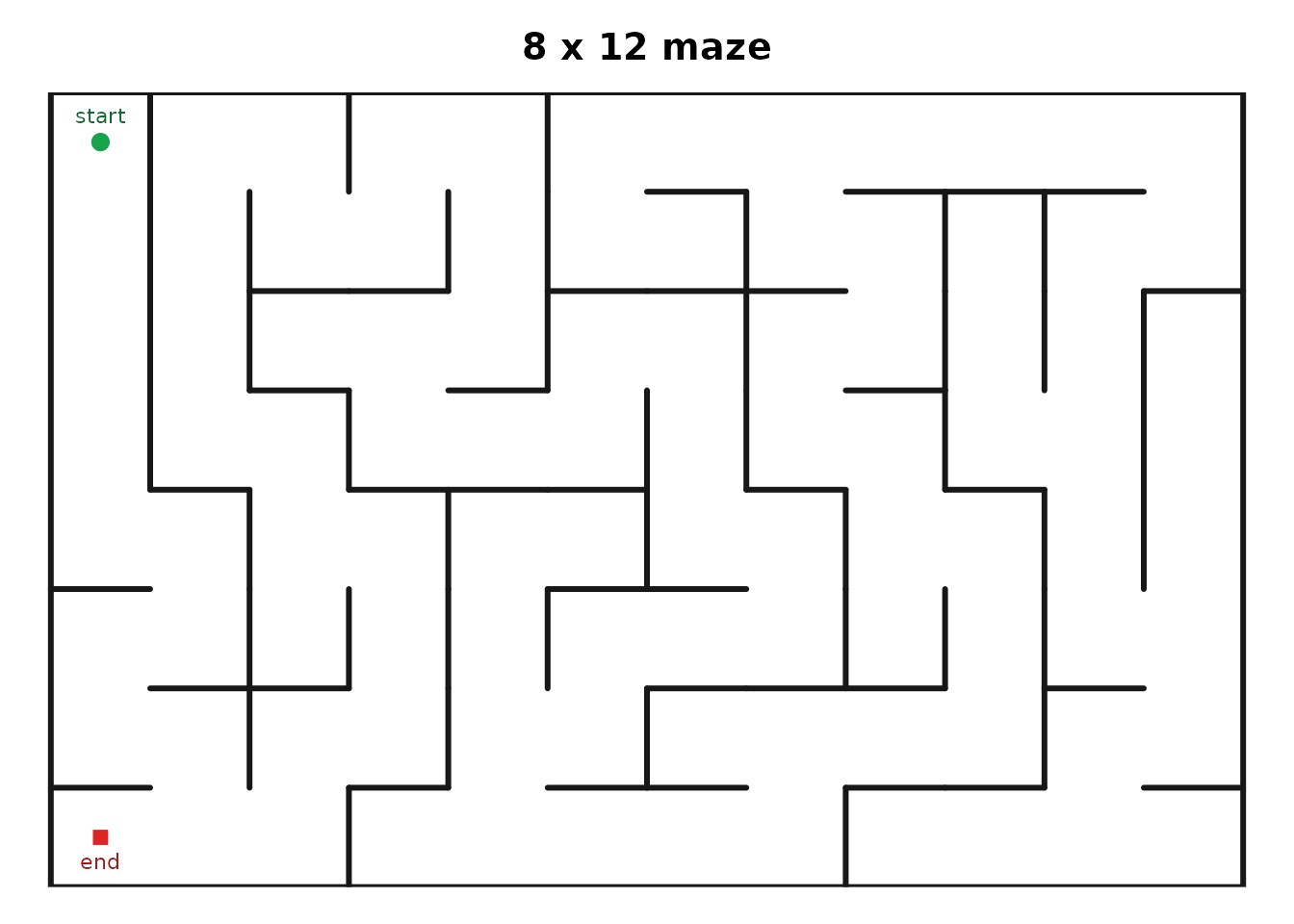
DFS is the only algorithm that produces a single contiguous walk, so
it is the only one that records traversal and
visitation_order. Those two fields are NULL
for every other algorithm, and plot_maze(show_path = TRUE)
is therefore available only for DFS mazes.
The other four algorithms
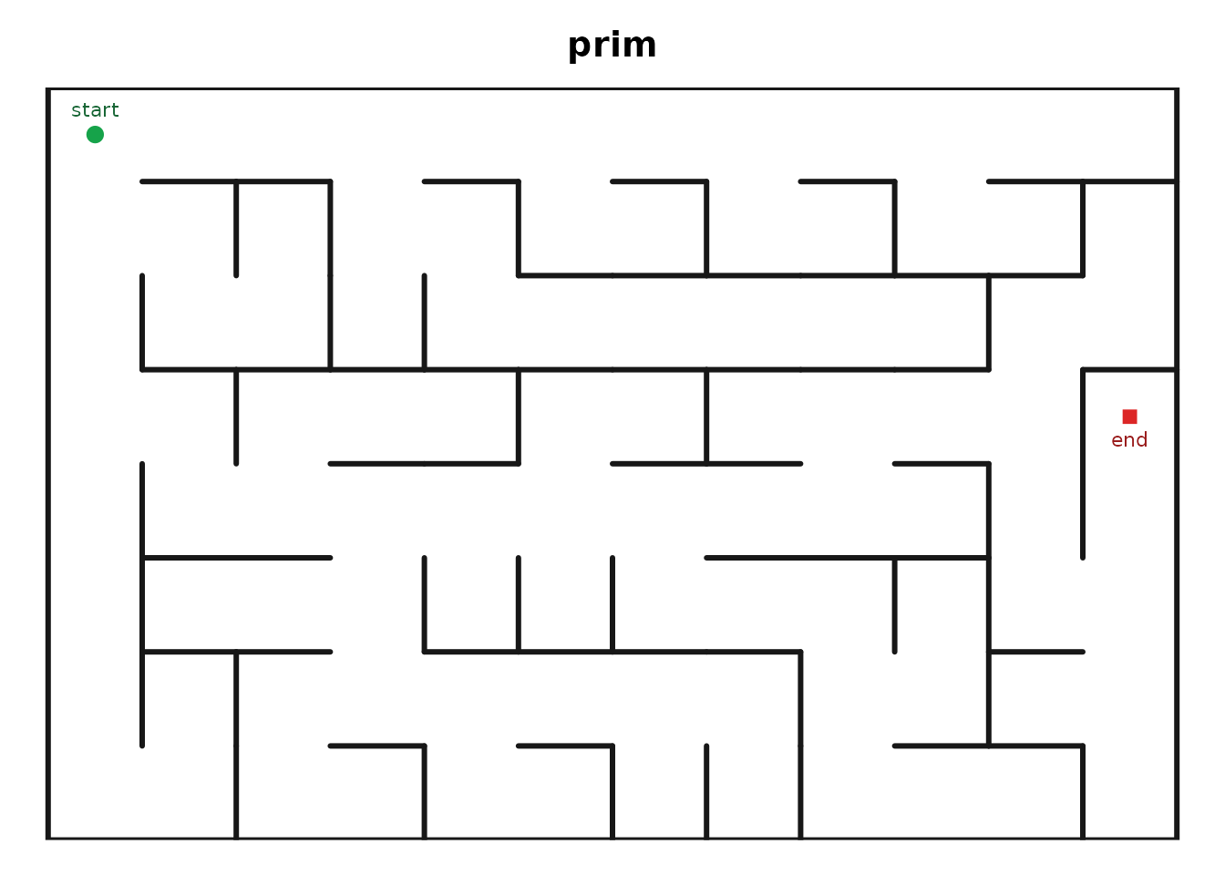
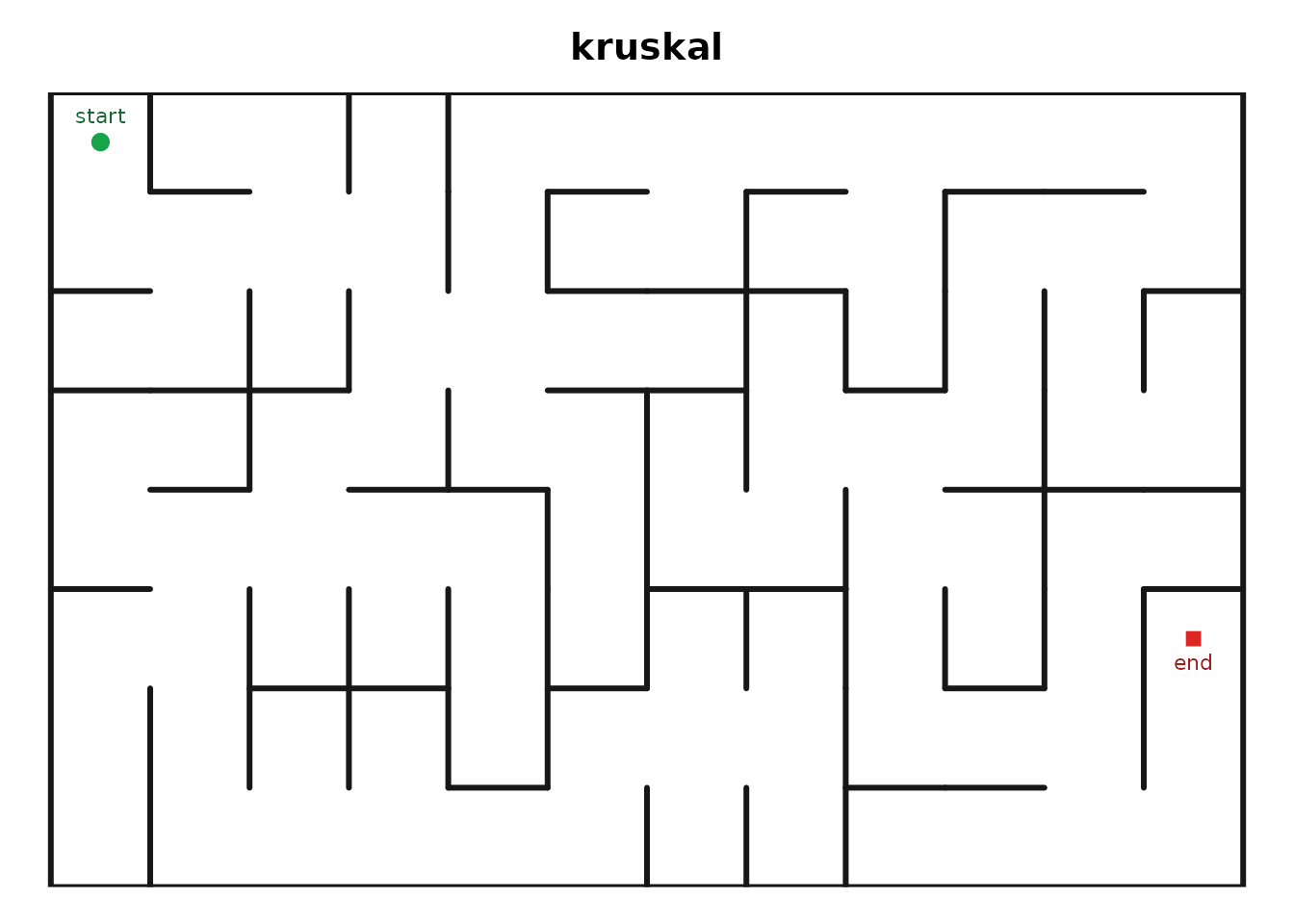
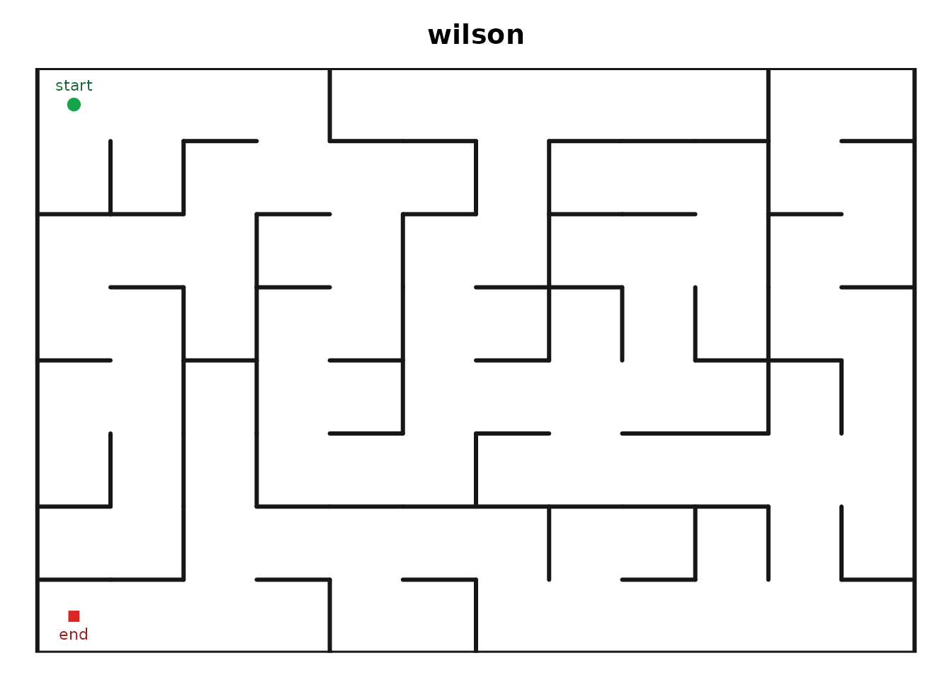
for (algo in c("prim", "kruskal", "wilson", "eller")) {
  plot_maze(
    generate_maze(8, 12, seed = 42, algorithm = algo),
    main = algo
  )
}
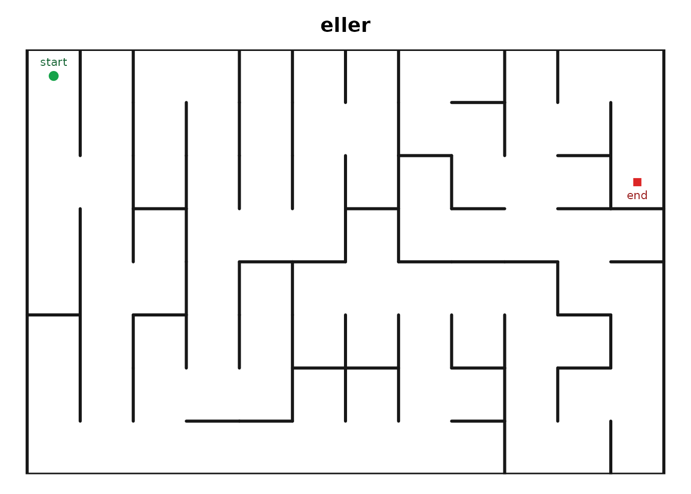
-
"prim"grows one tree outward fromstart, repeatedly carving a uniformly random wall on the frontier between the tree and the rest of the grid. The result branches evenly and is full of short dead ends – visually the opposite of DFS. -
"kruskal"shuffles every internal wall and carves each one whose two sides still belong to different components, tracked with a union-find. It has no bias towardstartat all, since it never looks at where the maze began. -
"wilson"builds a uniform spanning tree using loop-erased random walks: every perfect maze on the grid is equally likely. That statistical purity costs time, because the early walks wander a long way before they find the tree. -
"eller"sweeps one row at a time, merging cells into sets and carrying only a single row of state. It is the algorithm to reach for when the grid is too tall to hold in memory at once.
Why the result is a perfect maze
Each algorithm reaches the same invariant by a different argument, but the outcome is identical: no carved passage ever joins two cells that were already connected, and carving continues until everything is connected. A connected graph without cycles is a tree, so there is exactly one simple route between any pair of cells.
For a maze with rows × columns cells, the generator creates exactly one fewer unique passage than the number of cells.
length(maze$passages)
#> [1] 95
maze$rows * maze$cols - 1
#> [1] 95
Every maze also records carve_order, the passages in the
order they were opened. That is what animate_maze()
replays, and it is defined for all five algorithms – watching Prim
spread outward next to Wilson’s disconnected fragments snapping together
is the clearest way to see the difference.
Adding loops
open_walls breaks the invariant on purpose. After
generation, each remaining internal wall is independently removed with
the given probability, braiding the maze:
braided <- generate_maze(8, 12, seed = 42, open_walls = 0.3)
braided
#> <maze> 8 x 12
#>   algorithm: dfs
#>   start: (1, 1)
#>   end:   (8, 1)
#>   cells: 96
#>   loops: 19 walls removed (p = 0.3)
A braided maze is no longer a tree, so routes are no longer unique – which is exactly what makes it interesting to search.
Finding a route
solve_maze() searches the passage graph, with
algorithm choosing between three classic strategies:
-
"astar"(the default) is goal-directed. Manhattan distance is an admissible heuristic because maze movement is orthogonal and every step costs the same, so the path it returns is guaranteed shortest. -
"dijkstra"is the same search with the heuristic dropped: it expands uniformly outward fromstart, ignoring whereendis. -
"bfs"is the unweighted special case, a plain FIFO queue. It expands in rings of equal distance, and requires every step to cost the same.
solution <- solve_maze(maze)
head(solution)
#>   row column
#> 1   1      1
#> 2   2      1
#> 3   3      1
#> 4   4      1
#> 5   5      1
#> 6   5      2
plot_maze(maze, solution = solution)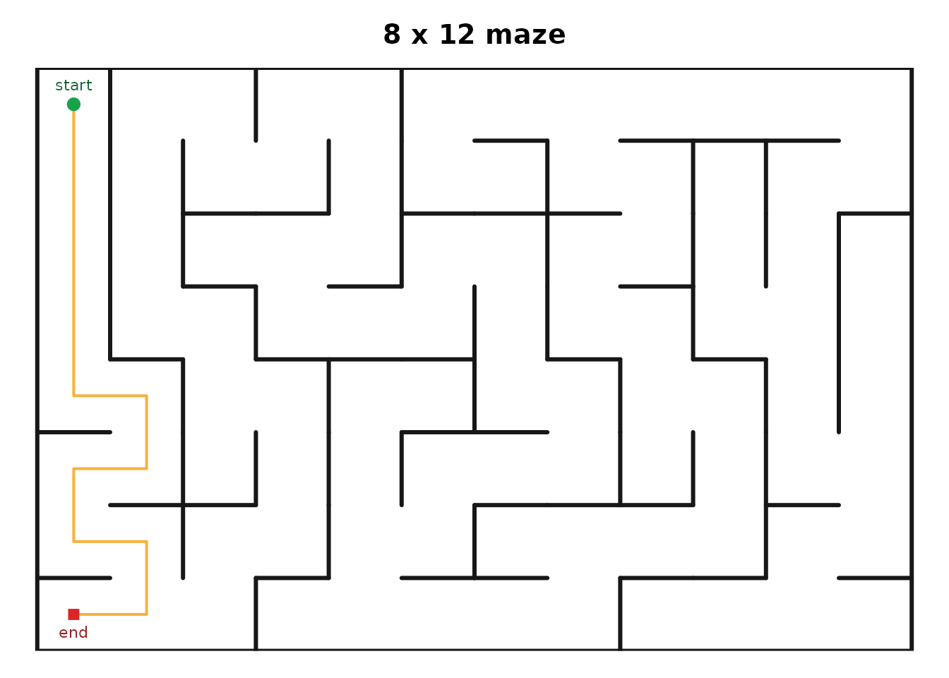
All three return a shortest route; what differs is how much of the
maze they touch getting there. trace = TRUE records every
expansion, which is both what animate_solution() replays
and an easy way to count the work:
big <- generate_maze(40, 40, seed = 123, algorithm = "kruskal")

vapply(c("astar", "dijkstra", "bfs"), function(algo) {
  traced <- solve_maze(big, algorithm = algo, trace = TRUE)
  length(attr(traced, "search_trace")$steps)
}, integer(1))
#>    astar dijkstra      bfs
#>     1303     1600     1600
The heuristic is what separates A-star from the other two. Note that
the gap depends entirely on how far apart start and
end are: for algorithm = "dfs" the end cell is
the last cell the walk visited, which frequently lands close to the
start, and then all three algorithms do nearly the same work. The other
four algorithms instead place end at the cell furthest from
start, which is why the comparison above uses one of
them.
solve_maze() also accepts a matrix in which selected
values represent walkable cells. When diagonal movement is enabled,
Euclidean distance and diagonal step costs are used so the search still
returns a shortest path – and because those steps no longer cost the
same, "bfs" rejects that combination.