Solve a maze or walkable matrix with graph search
solve_maze.RdFor a maze object, the function follows its passages. A numeric or
logical matrix can also be supplied, in which case cells matching
walkable may be crossed.
Arguments
- x
A
mazeobject or a matrix.- start, end
Integer vectors
c(row, column). For a maze, they default to its recorded start and end. They are required for a matrix.- walkable
Values considered walkable when
xis a matrix.- diagonal
Allow diagonal movement for a matrix. Maze passages are always orthogonal. Note that
algorithmvalues that require uniform step costs ("bfs"and"bidirectional") rejectdiagonal = TRUEon a matrix (diagonal moves costsqrt(2), not 1); use"dijkstra","astar","bidirectional_dijkstra", or"bidirectional_astar"instead, all of which handle non-uniform step costs correctly.algorithm = "wall_follower"also rejectsdiagonal = TRUEbecause following a wall relies on the four cardinal turn directions.- trace
Record the state of the search so that it can be replayed. The trace is attached to the result as the
search_traceattribute and is whatanimate_solution()renders. Each recorded step also carriesside,"forward"or"backward"for the three bidirectional algorithms (which frontier that expansion belongs to) and"none"for every other algorithm.- algorithm
Search algorithm to use, one of
"astar"(the default),"dijkstra","bfs","greedy","bidirectional","bidirectional_dijkstra","bidirectional_astar","wall_follower", or"dead_end_filling":"astar": goal-directed A* search. Its heuristic biases expansion towardsend, so it typically expands the fewest cells."dijkstra": uniform-cost search – the special case A* reduces to when the heuristic is dropped – expanding uniformly outward fromstartregardless of whereendis."bfs": the unweighted special case of Dijkstra, a plain FIFO-queue breadth-first search, only valid when every step has the same cost (always true for a maze; true for a matrix unlessdiagonal = TRUE)."greedy": Greedy Best-First search. Implemented by reusing the A* machinery with the path-cost-so-far (g) term forced to zero, so expansion is driven purely by the heuristic distance toend. It is usually fast but, unlike"astar", is not guaranteed to find the shortest path."bidirectional": breadth-first search run simultaneously fromstartand fromend, alternating one expansion per side, until the two frontiers meet. Requires uniform step costs, like"bfs"."bidirectional_dijkstra": bidirectional Dijkstra. Like"bidirectional"but weighted, so it also works with the non-uniform step costsdiagonal = TRUEgives a matrix. Critically, it does not stop at the first cell the two frontiers have in common: with non-uniform costs the first meeting is not necessarily on the shortest path, so it keeps track of the best complete path found so far (mu) and only stops once neither frontier can possibly improve on it."bidirectional_astar": NBA* (New Bidirectional A*, Pijls & Post, 2009), a goal-directed version of"bidirectional_dijkstra". The forward frontier's heuristic aims atendand the backward frontier's aims atstart(seeheuristic). Running plain A* from both ends and stopping at the first meeting point is not a correct shortest-path algorithm, even with admissible heuristics, because a heuristic admissible for one direction is generally not consistent with the other; NBA* avoids this with per-side pruning rules tied to the shared best-known path lengthmu, without needing to evaluate the heuristic across both frontiers at once."wall_follower": the classic hand-on-the-wall maze-walking rule (seehand). It never looks at the whole maze, only at which of the cardinal directions around the current cell are open, and so it does not generally find the shortest path. On a maze with loops (seeopen_wallsingenerate_maze()) it can fail to reachendentirely; seehandbelow for what happens in that case."dead_end_filling": iteratively "fills in" every dead end (any non-start, non-end cell with at most one still-open connection) until nothing more can be removed. On a perfect maze this leaves exactly the solution corridor, which is then walked directly. On a braided maze (loops present) dead-end filling alone cannot resolve the remaining loop(s), so the surviving cells are searched with breadth-first search to recover the shortest path.
- heuristic
The heuristic A*-family algorithms (
"astar","greedy","bidirectional_astar") use to estimate the remaining distance to the goal. Ignored (with a warning if set explicitly) by every other algorithm –"dijkstra"and"bidirectional_dijkstra"always use a heuristic of zero, and"bfs","bidirectional","wall_follower", and"dead_end_filling"use none at all. One of:"auto"(the default):"manhattan"for orthogonal movement (a maze, or a matrix withdiagonal = FALSE),"euclidean"for a matrix withdiagonal = TRUE. This is the heuristic every one of these algorithms has always used; passing"auto"(or omittingheuristic) reproduces that exact behaviour."manhattan":abs(dx) + abs(dy). Admissible for orthogonal movement, but not fordiagonal = TRUE: it charges 2 for a diagonal step that actually costssqrt(2), so it can overestimate the true remaining distance and A* is no longer guaranteed to return the shortest path.solve_maze()errors if"manhattan"is requested together withdiagonal = TRUE."euclidean": straight-line distance. Admissible fordiagonal = TRUE(it never overestimates the true cost) but looser than"octile"."octile":(dx + dy) + (sqrt(2) - 2) * min(dx, dy), the tight admissible heuristic for a grid where orthogonal steps cost 1 and diagonal steps costsqrt(2)– exactly this package's cost model for a matrix withdiagonal = TRUE."chebyshev":max(dx, dy). Admissible only when diagonal moves cost the same as orthogonal ones, which is not this package's cost model (diagonal moves costsqrt(2)here). Provided for experimentation; it will not generally yield shortest paths in this package and is not a safe default."zero": always 0, which turns A* into Dijkstra (and"bidirectional_astar"into"bidirectional_dijkstra").a function
function(position, target)returning a single finite, non-negative number, for a custom heuristic.positionandtargetare eachc(row, column);solve_maze()errors if the function ever returns something else.
- hand
Which wall the
"wall_follower"algorithm keeps a hand on, one of"left"(the default) or"right". Ignored by every other algorithm. Following a wall only reachesendwhenendactually lies along some wall reachable fromstart, which is always true on a perfect maze but not guaranteed on a braided one. To avoid looping forever on a maze with cycles, the walk is capped at4 * rows * colssteps; if it has not reachedendby then,solve_maze()emits a warning and returns a zero-row result (as if produced by.no_cells(), adapted to a data frame).
Value
A data frame with row and column, ordered from start to end
(or, only for "wall_follower" when it fails to reach end, a
data frame with zero rows – see hand). When trace = TRUE it
carries a search_trace attribute: a list with the grid dimensions,
the start and end cells, the algorithm used, and one
entry per expansion in steps, each holding the expanded cell
(current), the cells that it added to the frontier (opened),
and side ("forward", "backward", or "none";
see trace). For "wall_follower", each step is one move of the
walk: current is the cell just arrived at and opened holds
the single next cell the rule decides to move to (or no cells when the
walk is stuck or finished). For "dead_end_filling", the trace
begins with one step per cell filled in (current is the filled
cell, opened is always empty), followed by the ordinary
breadth-first-search steps (in the same shape as algorithm = "bfs")
over the cells that survived filling.
See also
animate_solution to render a traced search as a GIF.
Examples
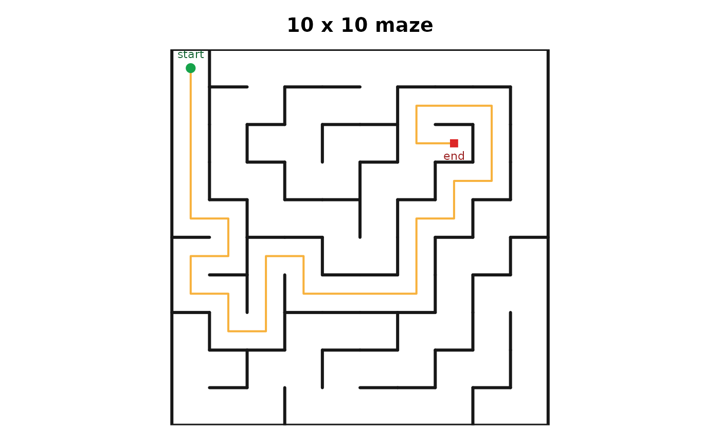
maze <- generate_maze(10, 10, seed = 42)
path <- solve_maze(maze)
plot_maze(maze, solution = path)
 # Compare how many cells each algorithm expands on the same maze.
expansions <- vapply(c("astar", "dijkstra", "bfs"), function(algo) {
solved <- solve_maze(maze, algorithm = algo, trace = TRUE)
length(attr(solved, "search_trace")$steps)
}, integer(1))
expansions
#> astar dijkstra bfs
#> 30 31 31